In a recent blog entry for my employer titled GeoMesa analytics in a Jupyter notebook, I wrote

As described on its home page, “The Jupyter Notebook is a web application that allows you to create and share documents that contain live code, equations, visualizations and explanatory text. Uses include: data cleaning and transformation, numerical simulation, statistical modeling, machine learning and much more.” Once you install the open source Jupyter server on your machine, you can create notebooks, share them with others, and learn from notebooks created by others. (You can also learn from others’ notebooks without installing Jupyter locally if those notebooks are hosted on a shared server.)

An animated GIF below that passage shows a sample mix of formatted text and executable Python code in a short Jupyter notebook, and it also demonstrates how code blocks can be tweaked, run in place, and build on previous code blocks. The blog entry goes on to describe how we at CCRi embedded Scala code in a Jupyter notebook to demonstrate the use of Apache Spark with the Hadoop-based GeoMesa spatio-temporal database to perform data analysis and visualization.

Jupyter supports over 40 languages besides Scala and Python, but not SPARQL. I realized recently, though, that with a minimum of Python code (Python being the original language for these notebooks; “Jupyter” was originally called “IPython”) someone who hardly knows Python can enter and run SPARQL queries in a Jupyter notebook.

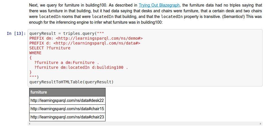
I created a Jupyter notebook that you can download and try yourself called JupyterSPARQLFun. If you look at the raw version of the file you’ll see a lot of JSON, but if you follow that link you’ll see that github renders the notebook the same way that a Jupyter server does, so you can read through the notebook and see all the formatted explanations with the code and the results.

If you did download the notebook and run it on a Jupyter server (and installed the rdflib and RDFClosure python libraries), you could edit the cells that have executable code, rerun them, and see the results, just like in the animated GIF mentioned above. In the case of this notebook, you’d be doing SPARQL manipulation of an RDF graph from your copy of the notebook. (I used the Anaconda Jupyter distribution. It was remarkably difficult to find out from their website how to start up Jupyter, but I did find out from the Jupyter Notebook Beginner Guide that you just enter “jupyter notebook” at the command line. When working with a notebook, you’ll also find this list of keyboard shortcuts to be handy.)

I won’t go into great detail here about what’s in the JupyterSPARQLFun notebook, because much of the point of these notebooks is that their ability to mix formatted text with executable code lets people take explanation of code to a new level. So, to find out how I got SPARQL and inferencing working in the notebook, I recommend that you just read the explanations and code that I put in it.

I mentioned above how you can learn from others’ notebooks; some nice examples accompany the Data School Machine Learning videos on YouTube. These videos demonstrate various concepts by adding and running code within notebooks, adding explanatory text as well along the way. Because I could download the finished notebooks created in the videos, I could run all the example code myself, in place, with no need to copy it from one place and paste it to another. I could also tweak the code samples to try different variations, which made for some much more hands-on learning of the machine learning concepts being demonstrated.

That experience really showed me the power of Jupyter notebooks, and it’s great to see that with just a little setup Python code, we can do SPARQL querying and RDF inferencing inside these notebooks as well.